Module 7: Choropleth and Proportional Symbol Mapping

This week's lab was to teach us how to select an appropriate color scheme for a choropleth map and the best legend layout to go with it.  The other part of the lab goal to learn how to use proportional or graduated symbols.

To create the map showing Europe's population density by country, adjusted the symbology to show quantities of population density.  The same was done for male and female population, but was normalized by population.  The other purpose of the map was to show wine consumption by country.  This step required using gradual symbols.  I decided to use gradual symbols because it was easier to differentiate from each class. 

This lab caused me to really worry about possibly lying about the data unintentionally.  I am eager to practice more data classification and symbology choices to see which will display a true and good map.

Module 6: Data Classification

Module 6 went through the different data classifications and compare and contrast the different classifications.  It also helped give experience on how best to symbolize or choose color schemes.

The map for this module displays four different data classification of the population of Escambia over the age of 65.  To display all of the types of data classification, three more data frames were added.  For each data frame I selected to show the data by quantities and changed how they were classified.  I selected natural breaks, standard deviation, equal interval, and quantiles for each data frame.  

I tried to pick a color scheme that would show the low classes and allow me to compare the data across the four maps.  I enjoyed how this lab allows you to see how data is classified can change what the data shows.  One map makes it seem like there is a high population of those 65 and older in one census tract, while another shows there is less.  Data classification can be used to show what you want to show and you hope people only try to show the true data.

GIS 4303 Week 6

This week's lab was the second half of working with projections and adding X, Y data to our map.

This map is of aerial photos of Escambia County of Florida.  The additional shapefiles of streets and counties need to have the projection changed to Florida Albers.  By doing this through the Project tool, the streets and aerial photos match up.

The next piece I have used at work and is very beneficial is adding points from X, Y data.  By adding this data and exporting it as a shapefile it places the storange tanks on to the map.  In order for the tanks to be in the right location, I had to reproject to WGS84.

I think this lab was good practice for what we will come across in the real world.  Data will be in different projections, but need to redefine it.  It shows how important it is to know details about your data so you can map accurately.

Module 5: Spatial Statistics

Module 5 was about understanding spatial statistics and learning how to apply the tools in ArcMap.  The tools helped find mean and median distribution of data.  Also able to display the data through a histogram, QQ plot, and learn to find outliers with spatial statistic tools.

One of the exercises used the mean center tool to show the mean location of the data  with a symbol.  I then used the median center tool to display the median location of the data.  This shows the clusters in certain countries have a greater affect on the median. To see the direction of the distribution used the spatial analysis toolbox.  As you can see on the map, it is an east-west orientation.  The large ellipsoid shows there is a large variation between the locations of the data.

It is important to understand how to use the data and what it is saying.  Understanding statistics will help aid in the analysis of data.

GIS 4303 Week 5

Week 5 covered projection, how to reproject and how to adjust coordinate systems for different layers.  Also learned how to map multiple data frames.

This map is showing three different projections: UTM, Albers, and State Planar.  To create this map, three separate data frames were required.  I started with one shapefile of Florida and used the Project tool to change the projection into two other coordinate systems creating new layers.  Looking at the map of all three, it is clear to see how Florida changes under the projections.  The area of the four specific counties have changed from projection to projection.  The changes in area can also be seen in the legends.

This lab is one of the most important to understand.  Projection is key to creating an accurate map.  If the projection is off, locations won't be portrayed correctly.  Different data will be in various projections which is why it is important to learn how to change the coordinate system to a usable one.

Module 4: Typology

Week 4's map was to teach us about typology and show an understanding proper placement of map elements.

This map is of the Marathon, Florida of the Florida Keys.  The major cities were labeled, along with a state park and airport.  Another key element to label was each key along with the bodies of waters.  All of the edits to the map were created in CorelDraw.  The main tools used were import, text tool, curve tool, and adjusting properties.  I had to use lines to label the cities and keys since the labels were too large to place on the land. 

I had to think carefully of font size and position to make sure the map didn't become too crowded or hard to read.  The different font sizes help the viewer determine which labels are the most important.  I also kept the font san serif to help make it be more readable. 

I think this lab was rather challenging to create a map that was easy to read and display all the elements.  I feel if I was able to create a good map in this lab, I should be able to tackle most.

GIS 4303 Week 4

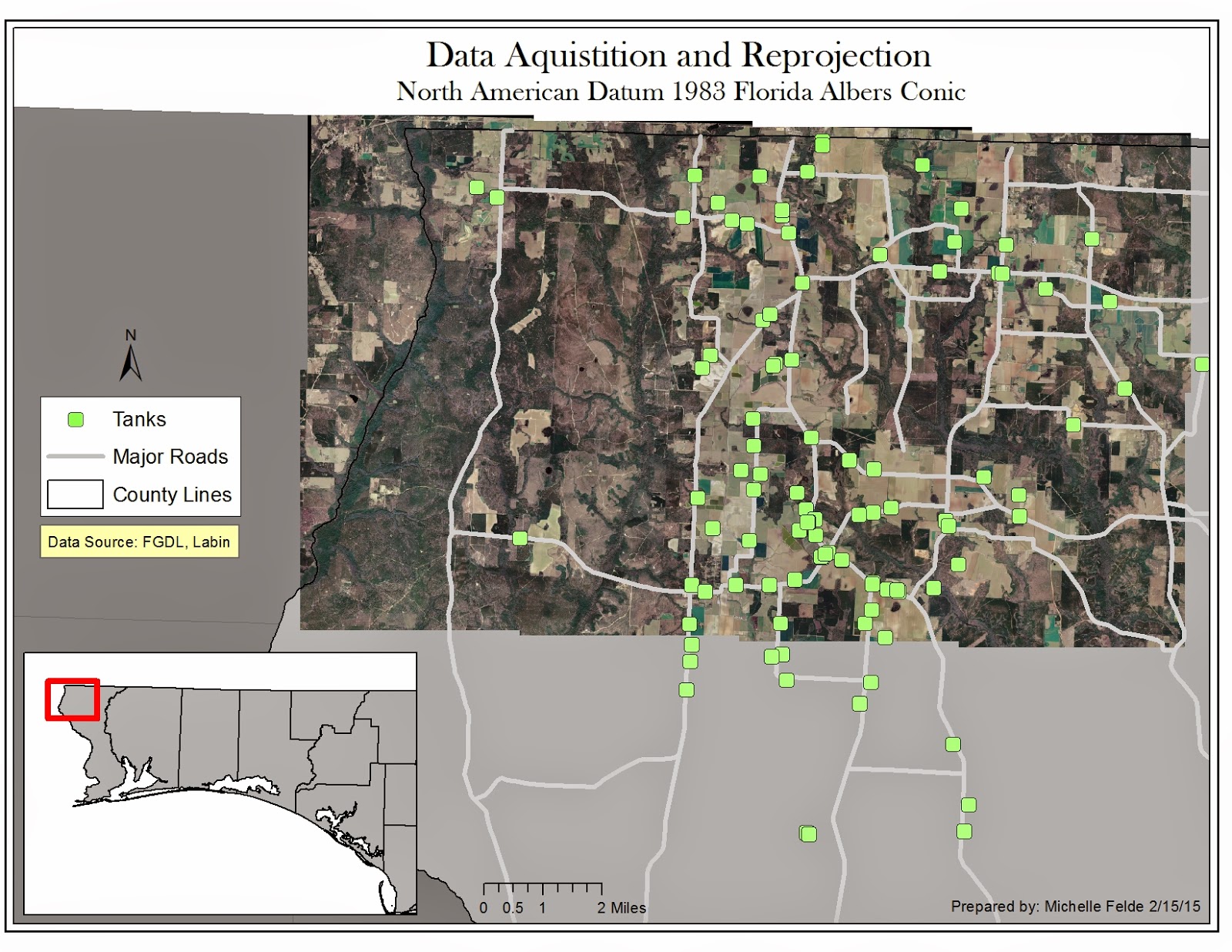
Week 4 lab was about sharing maps on ArcGIS online and map packaging.  The first part of the lab was learning about map packaging and the different types of packaging.  I adjusted the data in ArcGIS and logged into ArcGIS online through ArcMap.  To have the map contents in my content, select Share As.  From this pop up box the item description, tags, credits, and summary.  I analyzed the share to make sure there were no errors and then selected Share. See Image 1 below.

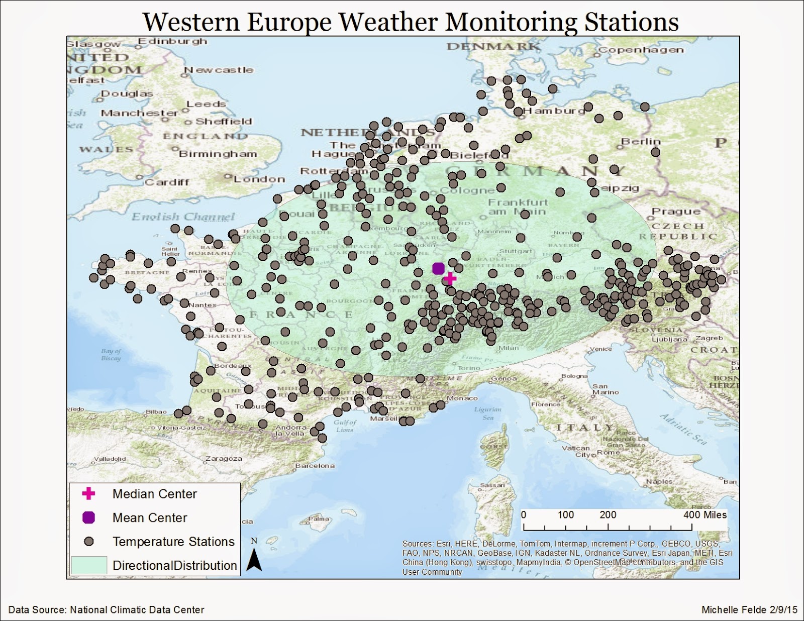
The second part of the lab consisted of optimizing map package.  After adding the data, one layer would be a generalized layer while the other detailed.  In both layers I adjusted the symbology and set the scale from ArcGIS online to show the detailed trees if zoomed in at a large scale.  On the generalized layer, I adjusted the properties so the trees would be smaller when zoomed out, but invisible when zoomed at the large scale.  I then followed the steps from the previous section of selecting Share As and added the item description, tags, credits, and uploaded the text file for additional details.  See image 2 below.

Learning to share map packages seems for powerful and something to possibly use at my work.  It would allow for people to see the map created and work with it.  It also amazes me how much data you can share and use from others due to this tool. 





Image 1



Image 2