GIS 4303: Final Project

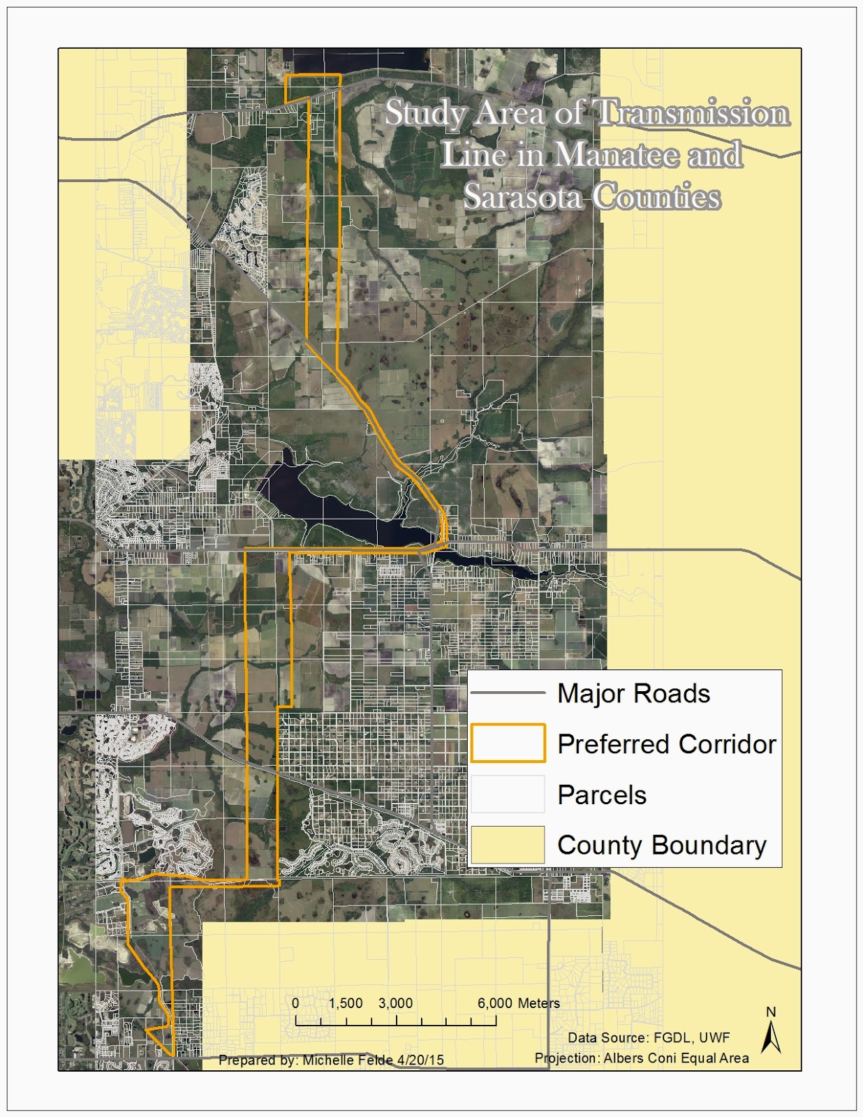
The final lab objective was to expose us to the experience of being a GIS professional.  The client was Florida Power & Light and they needed to install a new transmission line.  In order to meet FPL's objectives, it was important to apply all that was learned through the course.  It required gathering data, preforming buffers, select by attributes and more.

The main component of the lab consisted of seeing what land types, how many houses, how many schools, and cost that falls with in the preferred corridor for the transmission line.  To do this, it was necessary to clip land types to the corridor and calculate acres.  Creating a buffer around the preferred corridor also helped to see future impact on the community.  To count the numbers that fell within the corridor and buffer, heads up digitizing was a key part of the process. 

This lab was challenging, but in a great way.  I think it really helped me see what would be expected of me in the workplace for GIS analysts.  I think it also helped me show myself what I have really learned through this class.  Having to think of how to get a specific end result, really opens your eyes to various ways in ArcMap. 

To see my final maps and presentation click on the links below:

 http://students.uwf.edu/mf34/Intro2GIS/Planning_the_Bobwhite-Manatee_Transmission_Line.pdf
 

 http://students.uwf.edu/mf34/Intro2GIS/Slide_by_Slide_Commentary.pdf
 

 

 

 

 

GIS 4303: Week 13

Week 13's lab introduced georeferencing which allows users to take a non-spatial referenced raster and have it line up with features.  By doing this, it gives the raster a spatial reference.  Also learned to create a multi ring buffer and the editor toolbar.  Another piece of the lab was learning to use ArcScene.  In ArcScene, user is able to create a 3D map and learn how to adjust the layers.

The first map I created using the georeferencing tool.  To do this, I had to pick points on the raster image and match the location on the vector polygon.  One key thing was keeping a low RMS error and making sure the placement looked accurate.  Some polygons and lines were missing, so I used the editor toolbar to create new features.  To show the protection shown of the eagle's next, had to create a multi ring buffer.

The second map I created, used the building layer in ArcScene.  In ArcScene, I was able to show the buildings in 3D.  There are quite a few things to adjust in ArcScene, like base height and vertical exaggeration.  This map shows the UWF campus buildings, in 3D with the roads called out.

Module 12: Google Earth Mapping

Module 12 of Cartography class showed a way to apply layers and maps from ArcMap to Google Earth.  By converting layers and maps into KML files, they open n Google Earth and the fun can really begin.  I have only used Google Earth a few times and now knowing how to create a tour, I can really see how powerful this could be to present data.

The screenshot below shows what adding a KML map to Google Earth looks like.  The screenshot shows the southern part of Florida.  You can see more of the state, but more data with the added map.  You can see where how population density is and then zoom into Google Earth.  I converted a layer file of the counties and a created map to KML to added it to Google Earth.  From there you can explore Florida and the various cities of interest.  It is a great way to interact with your data and the map itself.  Not only can you explore your area of interest, but expand and compare which would be more difficult in ArcMap.  Also, creating a tour allows the creator to show the viewer key places or data.

Sadly, don't see how I can use this at my current job.  As I work to complete my course, can't wait to search for a job that will let me apply all that I am learning.

Module 11: 3D Mapping

The objectives of this lab was to understand the data needed to create a 3D map.  With the data, learn to map 3D raster and vector data.  Another objective was convert 2D features to 3D, along with using ArcScene and Analyst Extension.  Adjusting base height and rendering was key in creating a well made map.  Exporting the data as a .kmz allowed for us to interact with it in Google Earth.

3D mapping has pros and cons.  A map in 3D is less boring and allows for more interaction.  It can show an area in a different way than a map that is flat.  A lot of different objects can be portrayed.  3D maps add an element of art and so many options to portray the map elements.

It is great for showing different landscapes and various options.  3D maps would be great for urban planning and presenting plans.  The data can also be shared.

One con of 3D mapping is learning to use the tools.  It also seems to take longer to process.  3D maps could be harder to interpret.  In order to map 3D, need to have z values which might not always be available.

GIS 4303: Week 12

This week's lab covered how to create an address locator, geocode addresses, and create a route analysis.  In addition to creating a route analysis, also found optimal route.

After downloading the census data, I opened the data in ArcCatalog to create the address locator.  I had to choose a reference field, selected dual range, and populate certain fields.  In ArcMap, added the feature class of addresses and selected Geocode Addresses.  I adjusted the minimum match requirement and geocoded the addresses.  I rematched the unmatched addresses by either picking address on the map or looking at the possible matches in the interactive box.

To find the best route of the Emergency Medical Service locations, I had to added stops to the map by using the Network Analyst toolbar.  I added three stops and used the Network Analysis to calculate the route.  Before that happened, I adjusted the analysis settings to find the best route in minutes, set up restrictions, and checked to avoid invalid locations.

The second part of the lab involving Model Builder.  This gave me good insight into how a model is crated and that is can be used to run multiple tools.  It seems like it would greatly save time and be used as notes to remember how a map was created.