Module 8: Isarithmic Mapping

For module 8, we worked with continuous raster data.  With the data, it was also important to understand PRISM Interpolation Method.  With Isarithmic mapping, learning how to display continuous data is important.  We also learned another option for displaying the data through hyposemtric symbology and the legend that goes with it.  Within the maps, to help the viewer, we learned about adding contour lines.

The first map I prepared showed the data with continuous symbology.  This is done under the symbology tab of the layer's properties.  The symbology stayed as "stretched".  I added hillshade effect and adjusted the minimum and maximum.  I added a legend with the graphic being horizontal and used the legend properties to expand the length of the graphic.

The second map I prepared shows the data with hyposemtric symbology.  I first used the Int Spatial Analyst Tool to convert the raster values to integers for the contour lines.  I followed the same steps as the first map but used classes to symbolize the data.  I had the data broken up into 10 classes.  Next added contour lines using the Contour List tool. 

The maps show the annual precipitation of the state of Washington for 30 years.  The contour lines help make the changes in precipitation easier to see and help with analysis.

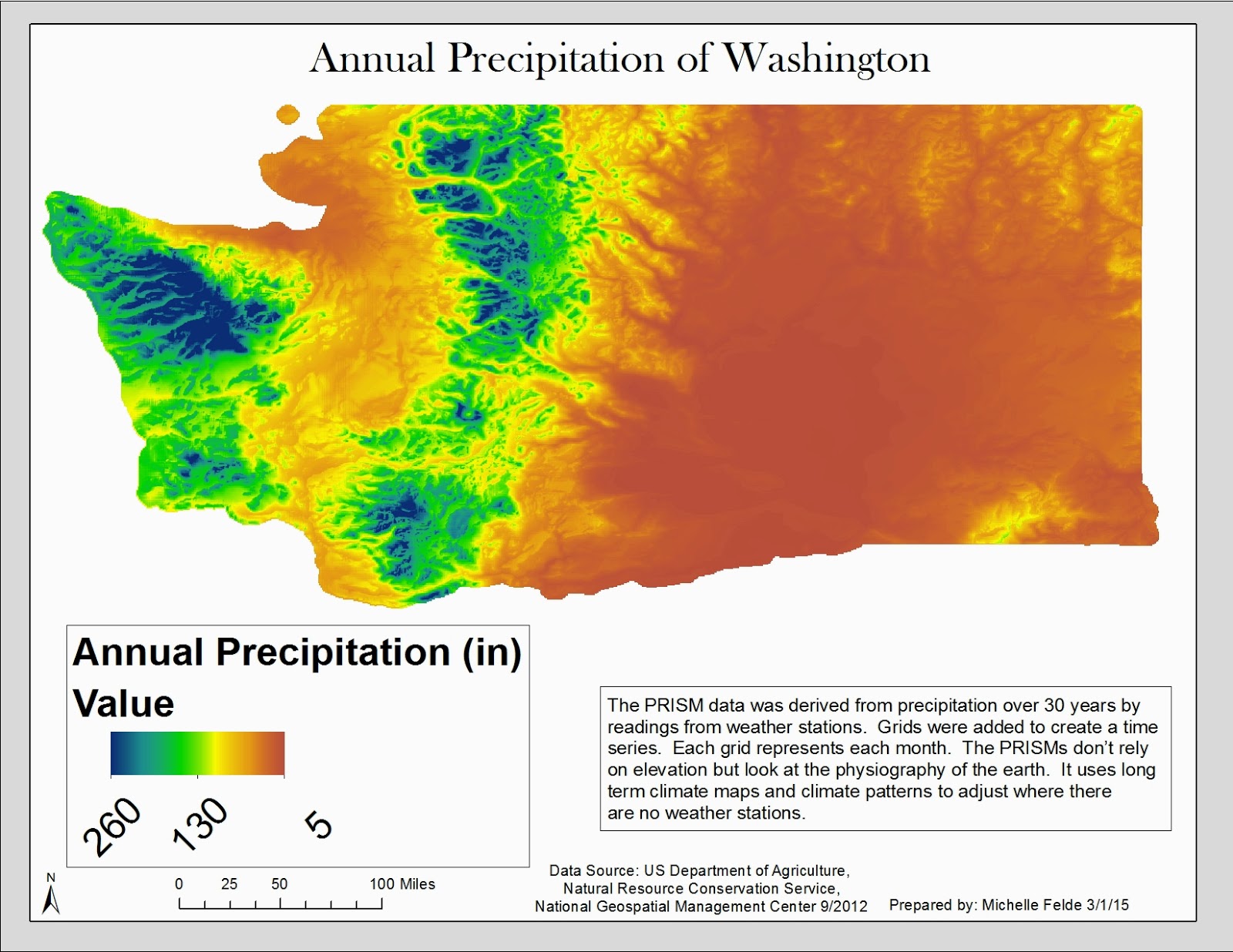Map 1

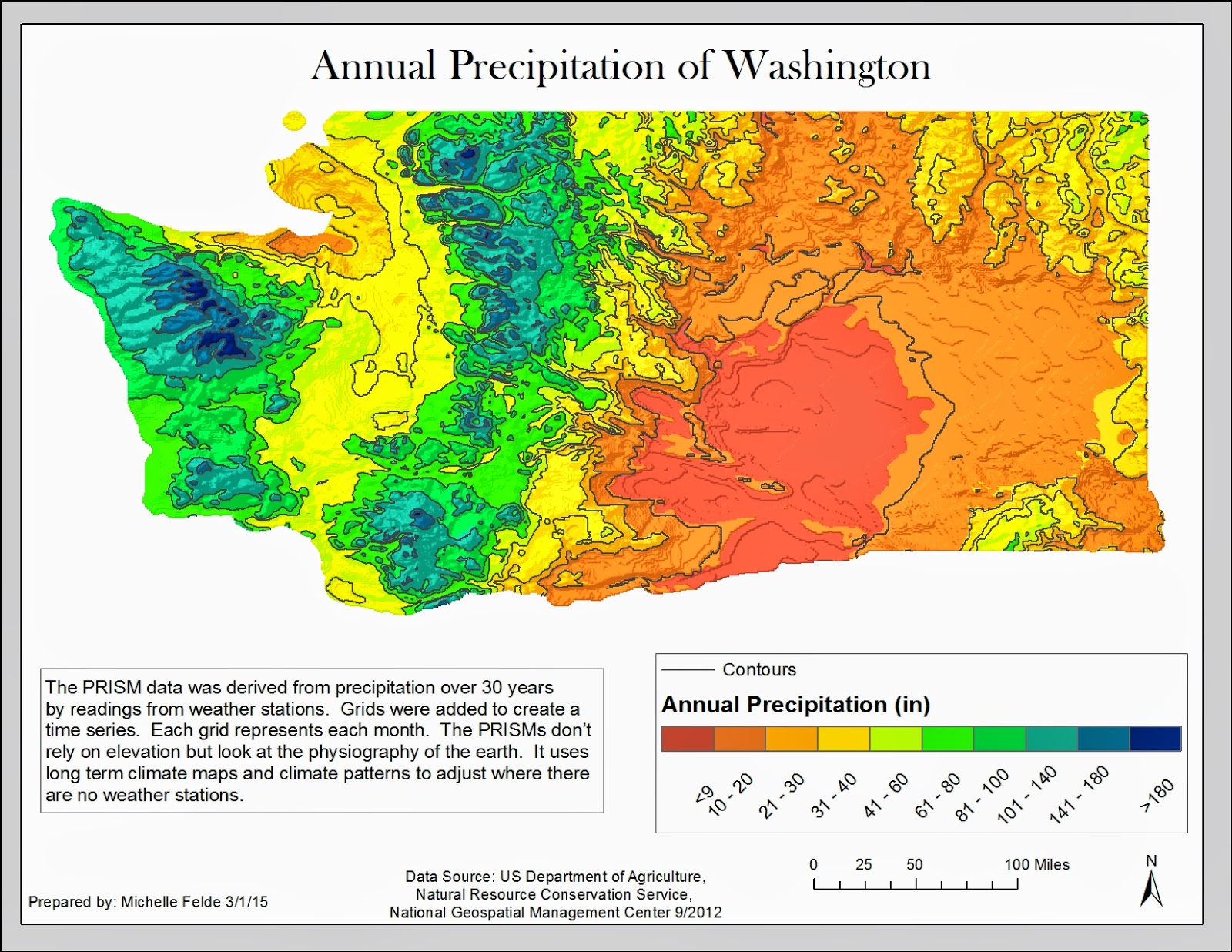Map 2